dim=4;
n=(dim+1)^2;
m=2*dim*(dim+1);
beta = 0.5;
alpha = 1;
G0 = 1;
C0 = [ 10 2 7 5 3;
8 3 9 5 5;
1 8 4 9 3;
7 3 6 8 2;
5 2 1 9 10 ];
wmax = 1;
CC = zeros(dim+1,dim+1,dim+1,dim+1,m+1);
GG = zeros(dim+1,dim+1,dim+1,dim+1,m+1);
CC(:,:,:,:,1) = reshape( diag(C0(:)), dim+1, dim+1, dim+1, dim+1 );
zo13 = reshape( [1,0;0,1], 2, 1, 2, 1 );
zo24 = reshape( zo13, 1, 2, 1, 2 );
pn13 = reshape( [1,-1;-1,1], 2, 1, 2, 1 );
pn24 = reshape( pn13, 1, 2, 1, 2 );
for i = 1 : dim+1,
GG(dim/2+1,i,dim/2+1,i,1) = G0;
for j = 1 : dim,
node = 1 + j + ( i - 1 ) * dim;
CC([j,j+1],i,[j,j+1],i,node) = beta * zo13;
GG([j,j+1],i,[j,j+1],i,node) = alpha * pn13;
node = node + dim * ( dim + 1 );
CC(i,[j,j+1],i,[j,j+1],node) = beta * zo24;
GG(i,[j,j+1],i,[j,j+1],node) = alpha * pn24;
end
end
CC = reshape( CC, n*n, m+1 );
GG = reshape( GG, n*n, m+1 );
npts = 50;
delays = linspace( 50, 150, npts );
xdelays = [ 50, 100 ];
xnpts = length( xdelays );
areas = zeros(1,npts);
for i = 1 : npts + xnpts,
if i > npts,
xi = i - npts;
delay = xdelays(xi);
disp( sprintf( 'Particular solution %d of %d (Tmax = %g)', xi, xnpts, delay ) );
else,
delay = delays(i);
disp( sprintf( 'Point %d of %d on the tradeoff curve (Tmax = %g)', i, npts, delay ) );
end
cvx_begin sdp quiet
variable x(m)
variable G(n,n) symmetric
variable C(n,n) symmetric
dual variables Y1 Y2 Y3 Y4 Y5
minimize( sum( C(:) ) )
subject to
G == reshape( GG * [ 1 ; x ], n, n );
C == reshape( CC * [ 1 ; x ], n, n );
delay * G - C >= 0;
0 <= x <= wmax;
cvx_end
if i <= npts,
areas(i) = sum(x);
else,
xareas(xi) = sum(x);
disp( sprintf( 'Solution %d:', xi ) );
disp( 'Vertical segments:' );
reshape( x(1:dim*(dim+1),1), dim, dim+1 )
disp( 'Horizontal segments:' );
reshape( x(dim*(dim+1)+1:end), dim, dim+1 )
figure(xi+1);
A = -inv(C)*G;
B = -A*ones(n,1);
T = linspace(0,500,2000);
Y = simple_step(A,B,T(2),length(T));
indmax = 0;
indmin = Inf;
for j = 1 : size(Y,1),
inds = min(find(Y(j,:) >= 0.5));
if ( inds > indmax )
indmax = inds;
jmax = j;
end;
if ( inds < indmin )
indmin = inds;
jmin = j;
end;
end;
tthres = T(indmax);
GinvC = full( G \ C );
tdom = max(eig(GinvC));
elmore = max(sum(GinvC'));
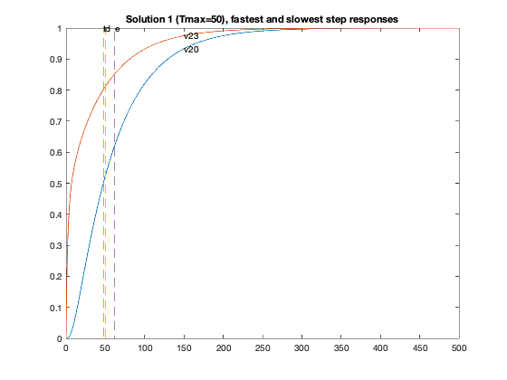
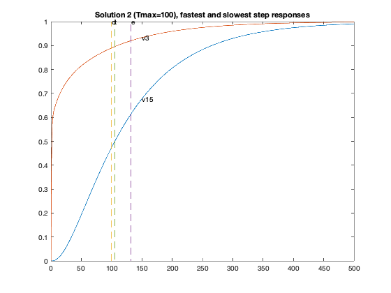
hold off; plot(T,Y(jmax,:),'-',T,Y(jmin,:)); hold on;
plot( tdom * [1;1], [0;1], '--', ...
elmore * [1;1], [0;1], '--', ...
tthres * [1;1], [0;1], '--');
axis([0 500 0 1])
text(tdom,1,'d');
text(elmore,1,'e');
text(tthres,1,'t');
text( T(600), Y(jmax,600), sprintf( 'v%d', jmax ) );
text( T(600), Y(jmin,600), sprintf( 'v%d', jmin ) );
title( sprintf( 'Solution %d (Tmax=%g), fastest and slowest step responses', xi, delay ) );
end
end;
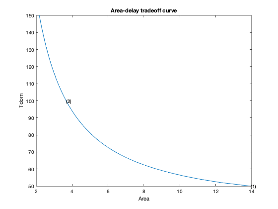
figure(1)
ind = isfinite(areas);
plot(areas(ind), delays(ind));
xlabel('Area');
ylabel('Tdom');
title('Area-delay tradeoff curve');
hold on
for k = 1 : xnpts,
text( xareas(k), xdelays(k), sprintf( '(%d)', k ) );
end
Point 1 of 50 on the tradeoff curve (Tmax = 50)
Point 2 of 50 on the tradeoff curve (Tmax = 52.0408)
Point 3 of 50 on the tradeoff curve (Tmax = 54.0816)
Point 4 of 50 on the tradeoff curve (Tmax = 56.1224)
Point 5 of 50 on the tradeoff curve (Tmax = 58.1633)
Point 6 of 50 on the tradeoff curve (Tmax = 60.2041)
Point 7 of 50 on the tradeoff curve (Tmax = 62.2449)
Point 8 of 50 on the tradeoff curve (Tmax = 64.2857)
Point 9 of 50 on the tradeoff curve (Tmax = 66.3265)
Point 10 of 50 on the tradeoff curve (Tmax = 68.3673)
Point 11 of 50 on the tradeoff curve (Tmax = 70.4082)
Point 12 of 50 on the tradeoff curve (Tmax = 72.449)
Point 13 of 50 on the tradeoff curve (Tmax = 74.4898)
Point 14 of 50 on the tradeoff curve (Tmax = 76.5306)
Point 15 of 50 on the tradeoff curve (Tmax = 78.5714)
Point 16 of 50 on the tradeoff curve (Tmax = 80.6122)
Point 17 of 50 on the tradeoff curve (Tmax = 82.6531)
Point 18 of 50 on the tradeoff curve (Tmax = 84.6939)
Point 19 of 50 on the tradeoff curve (Tmax = 86.7347)
Point 20 of 50 on the tradeoff curve (Tmax = 88.7755)
Point 21 of 50 on the tradeoff curve (Tmax = 90.8163)
Point 22 of 50 on the tradeoff curve (Tmax = 92.8571)
Point 23 of 50 on the tradeoff curve (Tmax = 94.898)
Point 24 of 50 on the tradeoff curve (Tmax = 96.9388)
Point 25 of 50 on the tradeoff curve (Tmax = 98.9796)
Point 26 of 50 on the tradeoff curve (Tmax = 101.02)
Point 27 of 50 on the tradeoff curve (Tmax = 103.061)
Point 28 of 50 on the tradeoff curve (Tmax = 105.102)
Point 29 of 50 on the tradeoff curve (Tmax = 107.143)
Point 30 of 50 on the tradeoff curve (Tmax = 109.184)
Point 31 of 50 on the tradeoff curve (Tmax = 111.224)
Point 32 of 50 on the tradeoff curve (Tmax = 113.265)
Point 33 of 50 on the tradeoff curve (Tmax = 115.306)
Point 34 of 50 on the tradeoff curve (Tmax = 117.347)
Point 35 of 50 on the tradeoff curve (Tmax = 119.388)
Point 36 of 50 on the tradeoff curve (Tmax = 121.429)
Point 37 of 50 on the tradeoff curve (Tmax = 123.469)
Point 38 of 50 on the tradeoff curve (Tmax = 125.51)
Point 39 of 50 on the tradeoff curve (Tmax = 127.551)
Point 40 of 50 on the tradeoff curve (Tmax = 129.592)
Point 41 of 50 on the tradeoff curve (Tmax = 131.633)
Point 42 of 50 on the tradeoff curve (Tmax = 133.673)
Point 43 of 50 on the tradeoff curve (Tmax = 135.714)
Point 44 of 50 on the tradeoff curve (Tmax = 137.755)
Point 45 of 50 on the tradeoff curve (Tmax = 139.796)
Point 46 of 50 on the tradeoff curve (Tmax = 141.837)
Point 47 of 50 on the tradeoff curve (Tmax = 143.878)
Point 48 of 50 on the tradeoff curve (Tmax = 145.918)
Point 49 of 50 on the tradeoff curve (Tmax = 147.959)
Point 50 of 50 on the tradeoff curve (Tmax = 150)
Particular solution 1 of 2 (Tmax = 50)
Solution 1:
Vertical segments:

ans =

    0.6555    0.4366    0.5234    0.4709    0.2363
    1.0000    0.8536    1.0000    0.9360    0.5700
    0.9233    0.2956    0.8004    1.0000    1.0000
    0.4130    0.1355    0.2672    0.6724    0.8867

Horizontal segments:

ans =

    0.1938    0.1436    0.0000    0.0000    0.0000
    0.0712    0.0633    0.0000    0.0000    0.0000
    0.0000    0.0000    0.0000    0.0945    0.1583
    0.0000    0.0000    0.0000    0.0865    0.0517

Particular solution 2 of 2 (Tmax = 100)
Solution 2:
Vertical segments:

ans =

    0.2688    0.0437    0.1712    0.1338    0.0736
    0.4135    0.0802    0.3064    0.2224    0.1485
    0.2576    0.0802    0.1120    0.3835    0.2816
    0.1344    0.0437    0.0245    0.2408    0.2453

Horizontal segments:

ans =

   1.0e-08 *

    0.2229    0.3083    0.2867    0.3101    0.2455
    0.1859    0.2203    0.2134    0.2305    0.1570
    0.2219    0.2200    0.2107    0.2218    0.1510
    0.2504    0.2411    0.2118    0.2290    0.2103