N = 4;
Cload = 12;
Vdd = 1.5;
NMOS = struct('R',0.4831, 'Cdb',0.6, 'Csb',0.6, 'Cgb',1, 'Cgs',1);
PMOS = struct('R',2*0.4831, 'Cdb',0.6, 'Csb',0.6, 'Cgb',1, 'Cgs',1);
Amax = 24;
wmin = 1;
Npoints = 25;
Amax = linspace(5,45,Npoints);
Dopt = [];
disp('Generating the optimal tradeoff curve...')
need_sedumi = strncmpi(cvx_solver,'sdpt',4);
if need_sedumi,
warning('This model does not converge with SDPT3... switching to SeDuMi.');
end
for k = 1:Npoints
fprintf(1,' Amax = %5.2f:', Amax(k));
cvx_begin gp quiet
if need_sedumi,
cvx_solver sedumi
end
variable w(N)
device(1:2) = PMOS; device(3:4) = NMOS;
for num = 1:N
device(num).R = device(num).R/w(num);
device(num).Cdb = device(num).Cdb*w(num);
device(num).Csb = device(num).Csb*w(num);
device(num).Cgb = device(num).Cgb*w(num);
device(num).Cgs = device(num).Cgs*w(num);
end
C1 = sum([device(1:3).Cdb]) + Cload;
C2 = device(3).Csb + device(4).Cdb;
Cin_A = sum([ device([2 3]).Cgb ]) + sum([ device([2 3]).Cgs ]);
Cin_B = sum([ device([1 4]).Cgb ]) + sum([ device([1 4]).Cgs ]);
R = [device.R]';
area = sum(w);
D1 = R(1)*(C1 + C2);
E1 = (C1 + C2)*Vdd^2/2;
D2 = R(2)*C1;
E2 = C1*Vdd^2/2;
E3 = C1*Vdd^2/2;
D4 = C1*R(3) + R(4)*(C1 + C2);
E4 = (C1 + C2)*Vdd^2/2;
D5 = C1*(R(3) + R(4));
E5 = (C1 + C2)*Vdd^2/2;
D6 = C1*R(3) + R(4)*(C1 + C2);
E6 = (C1 + C2)*Vdd^2/2;
minimize( max( [D1 D2 D4] ) )
subject to
area <= Amax(k);
w >= wmin;
cvx_end
fprintf(1,' delay = %3.2f\n',cvx_optval);
Dopt = [Dopt cvx_optval];
end
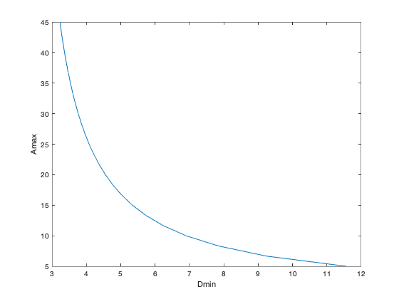
plot(Dopt,Amax);
xlabel('Dmin'); ylabel('Amax');
disp('Optimal tradeoff curve plotted.')
Generating the optimal tradeoff curve...
  Amax =  5.00: delay = 11.56
  Amax =  6.67: delay = 9.23
  Amax =  8.33: delay = 7.84
  Amax = 10.00: delay = 6.90
  Amax = 11.67: delay = 6.23
  Amax = 13.33: delay = 5.73
  Amax = 15.00: delay = 5.34
  Amax = 16.67: delay = 5.03
  Amax = 18.33: delay = 4.77
  Amax = 20.00: delay = 4.55
  Amax = 21.67: delay = 4.37
  Amax = 23.33: delay = 4.22
  Amax = 25.00: delay = 4.08
  Amax = 26.67: delay = 3.96
  Amax = 28.33: delay = 3.86
  Amax = 30.00: delay = 3.76
  Amax = 31.67: delay = 3.68
  Amax = 33.33: delay = 3.60
  Amax = 35.00: delay = 3.54
  Amax = 36.67: delay = 3.47
  Amax = 38.33: delay = 3.42
  Amax = 40.00: delay = 3.36
  Amax = 41.67: delay = 3.32
  Amax = 43.33: delay = 3.27
  Amax = 45.00: delay = 3.23
Optimal tradeoff curve plotted.