n = 4;
m = 6;
G = 0.1;
Co = 10;
wmax = 10.0;
alpha = [ 1.0, 1.0, 1.0, 1.0, 1.0, 1.0 ];
beta = [ 10, 10, 100, 1, 1, 1 ];
CC = zeros(n,n,m+1);
GG = zeros(n,n,m+1);
CC(3,3,1) = Co;
GG(1,1,1) = G;
CC(1,1,2) = + beta(1);
CC(2,2,2) = + beta(1);
GG(1,1,2) = + alpha(1);
GG(2,1,2) = - alpha(1);
GG(1,2,2) = - alpha(1);
GG(2,2,2) = + alpha(1);
CC(2,2,3) = + beta(2);
CC(3,3,3) = + beta(2);
GG(2,2,3) = + alpha(2);
GG(3,2,3) = - alpha(2);
GG(2,3,3) = - alpha(2);
GG(3,3,3) = + alpha(2);
CC(1,1,4) = + beta(3);
CC(3,3,4) = + beta(3);
GG(1,1,4) = + alpha(3);
GG(3,1,4) = - alpha(3);
GG(1,3,4) = - alpha(3);
GG(3,3,4) = + alpha(3);
CC(1,1,5) = + beta(4);
CC(4,4,5) = + beta(4);
GG(1,1,5) = + alpha(4);
GG(4,1,5) = - alpha(4);
GG(1,4,5) = - alpha(4);
GG(4,4,5) = + alpha(4);
CC(2,2,6) = + beta(5);
CC(4,4,6) = + beta(5);
GG(2,2,6) = + alpha(5);
GG(2,4,6) = - alpha(5);
GG(4,2,6) = - alpha(5);
GG(4,4,6) = + alpha(5);
CC(3,3,7) = + beta(6);
CC(4,4,7) = + beta(6);
GG(3,3,7) = + alpha(6);
GG(4,3,7) = - alpha(6);
GG(3,4,7) = - alpha(6);
GG(4,4,7) = + alpha(6);
CC = reshape(CC,n*n,m+1);
GG = reshape(GG,n*n,m+1);
npts = 50;
delays = linspace( 180, 800, npts );
xdelays = [ 200, 400, 600 ];
xnpts = length(xdelays);
areas = zeros(1,npts);
sizes = zeros(6,xnpts);
for i = 1 : npts + xnpts,
if i > npts,
xi = i - npts;
delay = xdelays(xi);
disp( sprintf( 'Particular solution %d of %d (Tmax = %g)', xi, xnpts, delay ) );
else,
delay = delays(i);
disp( sprintf( 'Point %d of %d on the tradeoff curve (Tmax = %g)', i, npts, delay ) );
end
cvx_begin sdp quiet
variable x(6)
variable G(n,n) symmetric
variable C(n,n) symmetric
minimize( sum( x ) )
subject to
G == reshape( GG * [ 1 ; x ], n, n );
C == reshape( CC * [ 1 ; x ], n, n );
delay * G - C >= 0;
0 <= x <= wmax;
cvx_end
if i <= npts,
areas(i) = cvx_optval;
else,
xareas(xi) = cvx_optval;
sizes(:,xi) = x;
figure(xi+1);
A = -inv(C)*G;
B = -A*ones(n,1);
T = linspace(0,1000,1000);
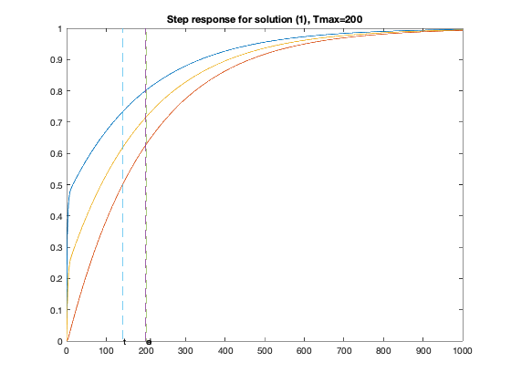
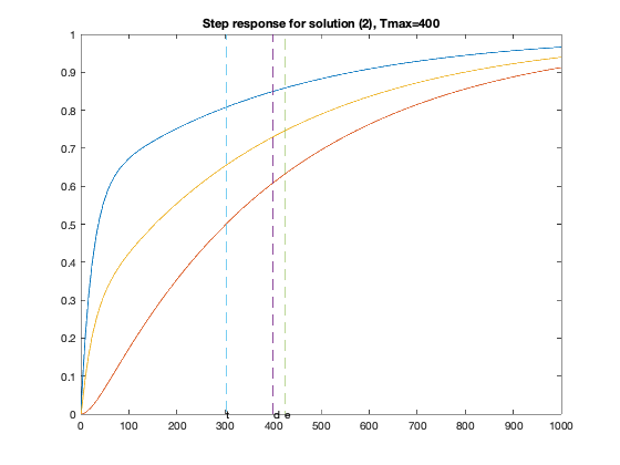
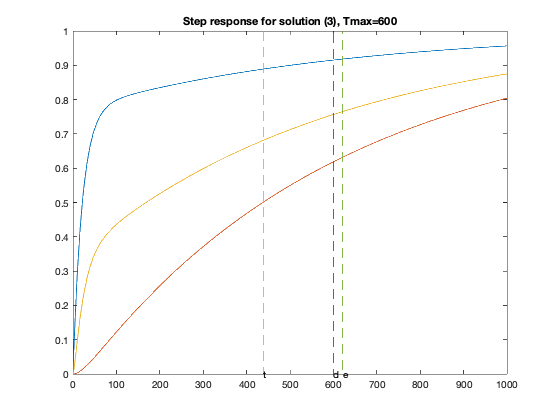
Y = simple_step(A,B,T(2),length(T));
hold off; plot(T,Y([1,3,4],:),'-'); hold on;
tthres=T(min(find(Y(3,:)>0.5)));
tdom=max(eig(inv(G)*C));
telm=max(sum((inv(G)*C)'));
plot(tdom*[1;1], [0;1], '--', telm*[1;1], [0;1],'--', ...
tthres*[1;1], [0;1], '--');
text(tdom,0,'d');
text(telm,0,'e');
text(tthres,0,'t');
title(sprintf('Step response for solution (%d), Tmax=%g', xi, delay ));
end
end
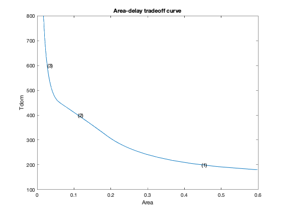
figure(1)
ind = isfinite(areas);
plot(areas(ind), delays(ind));
xlabel('Area');
ylabel('Tdom');
title('Area-delay tradeoff curve');
hold on
for k = 1 : xnpts,
text( xareas(k), xdelays(k), sprintf( '(%d)', k ) );
end
disp(['Three specific solutions:']);
sizes
Point 1 of 50 on the tradeoff curve (Tmax = 180)
Point 2 of 50 on the tradeoff curve (Tmax = 192.653)
Point 3 of 50 on the tradeoff curve (Tmax = 205.306)
Point 4 of 50 on the tradeoff curve (Tmax = 217.959)
Point 5 of 50 on the tradeoff curve (Tmax = 230.612)
Point 6 of 50 on the tradeoff curve (Tmax = 243.265)
Point 7 of 50 on the tradeoff curve (Tmax = 255.918)
Point 8 of 50 on the tradeoff curve (Tmax = 268.571)
Point 9 of 50 on the tradeoff curve (Tmax = 281.224)
Point 10 of 50 on the tradeoff curve (Tmax = 293.878)
Point 11 of 50 on the tradeoff curve (Tmax = 306.531)
Point 12 of 50 on the tradeoff curve (Tmax = 319.184)
Point 13 of 50 on the tradeoff curve (Tmax = 331.837)
Point 14 of 50 on the tradeoff curve (Tmax = 344.49)
Point 15 of 50 on the tradeoff curve (Tmax = 357.143)
Point 16 of 50 on the tradeoff curve (Tmax = 369.796)
Point 17 of 50 on the tradeoff curve (Tmax = 382.449)
Point 18 of 50 on the tradeoff curve (Tmax = 395.102)
Point 19 of 50 on the tradeoff curve (Tmax = 407.755)
Point 20 of 50 on the tradeoff curve (Tmax = 420.408)
Point 21 of 50 on the tradeoff curve (Tmax = 433.061)
Point 22 of 50 on the tradeoff curve (Tmax = 445.714)
Point 23 of 50 on the tradeoff curve (Tmax = 458.367)
Point 24 of 50 on the tradeoff curve (Tmax = 471.02)
Point 25 of 50 on the tradeoff curve (Tmax = 483.673)
Point 26 of 50 on the tradeoff curve (Tmax = 496.327)
Point 27 of 50 on the tradeoff curve (Tmax = 508.98)
Point 28 of 50 on the tradeoff curve (Tmax = 521.633)
Point 29 of 50 on the tradeoff curve (Tmax = 534.286)
Point 30 of 50 on the tradeoff curve (Tmax = 546.939)
Point 31 of 50 on the tradeoff curve (Tmax = 559.592)
Point 32 of 50 on the tradeoff curve (Tmax = 572.245)
Point 33 of 50 on the tradeoff curve (Tmax = 584.898)
Point 34 of 50 on the tradeoff curve (Tmax = 597.551)
Point 35 of 50 on the tradeoff curve (Tmax = 610.204)
Point 36 of 50 on the tradeoff curve (Tmax = 622.857)
Point 37 of 50 on the tradeoff curve (Tmax = 635.51)
Point 38 of 50 on the tradeoff curve (Tmax = 648.163)
Point 39 of 50 on the tradeoff curve (Tmax = 660.816)
Point 40 of 50 on the tradeoff curve (Tmax = 673.469)
Point 41 of 50 on the tradeoff curve (Tmax = 686.122)
Point 42 of 50 on the tradeoff curve (Tmax = 698.776)
Point 43 of 50 on the tradeoff curve (Tmax = 711.429)
Point 44 of 50 on the tradeoff curve (Tmax = 724.082)
Point 45 of 50 on the tradeoff curve (Tmax = 736.735)
Point 46 of 50 on the tradeoff curve (Tmax = 749.388)
Point 47 of 50 on the tradeoff curve (Tmax = 762.041)
Point 48 of 50 on the tradeoff curve (Tmax = 774.694)
Point 49 of 50 on the tradeoff curve (Tmax = 787.347)
Point 50 of 50 on the tradeoff curve (Tmax = 800)
Particular solution 1 of 3 (Tmax = 200)
Particular solution 2 of 3 (Tmax = 400)
Particular solution 3 of 3 (Tmax = 600)
Three specific solutions:

sizes =

    0.0000    0.0000    0.0000
    0.0000    0.0000    0.0000
    0.0000    0.0381    0.0273
    0.2303    0.0369    0.0000
    0.0000    0.0000    0.0000
    0.2156    0.0361    0.0000