Demo: Robust PCA using TFOCS
Download the SIAM_demo.m Matlab file and the escalator_data.mat data file if you would like to recreate this demo yourself.
This is a demo of Robust PCA (RPCA) using TFOCS. Since 2009, there has been much interest in this specific RPCA formulation (RPCA can refer to many different formulations; we will state our formulation precisely below), but most solvers assume equality constraints. One great feature of TFOCS is how easy it is to prototype new formulations, so we show here a formulation using inequality constraints.
The basic (equality constraint) RPCA formulation is (see here for references):\[
\min_{S,L} \|L\|_* + \lambda \|S\|_{\ell_1} \quad\textrm{subject to}\;L+S = X
\]The idea is that some object \(X\) can be broken into two components \(X=L+S\), where \(L\) is low-rank and \(S\) is sparse. To tease out this separation, RPCA penalizes \(\|L\|_*\) (the nuclear norm of \(L\)), which is a proxy for the rank of \(L\). We also penalize \(\|S\|_{\ell_1}\), which is just the sum of the absolute value of all the entries of the matrix \(S\); this is a proxy for the number of non-zero entries of \(S\).
The parameter \(\lambda\) is important, as it controls how much weight to put on \(S\) relative to \(L\). This parameter is not overly sensitive, and we picked the value used in this demo by a few quick rounds of trial-and-error.
Code by Stephen Becker, May 2011
Contents
- Inequality constraints
- Numerical demo
- show all together in movie format
- Is there a difference between the two versions?
Inequality constraints
In this demo, \(X\) is a video. In particular, each column of \(X\) is the set of \(mn\) pixels from a \(m\times n\) pixel frame of the video, reshaped so that it is now a vector instead of a matrix.
The particular video we use is not compressed using a video codec, so each frame of the video is stored. This leads to huge files, so to save a bit of space, the value of each pixel is stored as an 8 bit number, which means we can think of it as a value from \(0,1,2,\ldots,255\). Now, we may imagine that there is some “true” video where each pixel is a real number between \([0,255]\), and that we see a quantized version of it. It would be nice to apply RPCA to this true version instead of applying it to the quantized version. In particular, it is unlikely that the quantized version can be split nicely into a low-rank and sparse component. To account for this quantization, we will ask that \(S+L\) is not exactly equal to \(X\), but rather that \(S+L\) agrees with \(X\) up to the precision of the quantization. The quantization can induce at most an error of .5 in the pixel value (e.g. true value is 5.6, which is rounded to 6.0, so an error of .4; or a true value of 6.4, which is also rounded to 6.0, so also an error of 0.4). A nice way to capture this is via the \(\ell_\infty\) norm.
So, the inequality constrained version of RPCA uses the same objective function, but instead of the constraints \(L+S=X\), the constraints are \(\|L+S-X\|_{\ell_\infty} \le 0.5\).
Numerical demo
We demonstrate this on a video clip taken from a surveillance camera in a subway station. Not only is there a background and a foreground (i.e. people), but there is an escalator with periodic motion. Conventional background subtraction algorithms would have difficulty with the escalator, but this RPCA formulation easily captures it as part of the low-rank structure. The clip is taken from the data at this website (after a bit of processing to convert it to grayscale): http://perception.i2r.a-star.edu.sg/bk_model/bk_index.html
% Load the data:
load escalator_data % contains X (data), m and n (height and width)
X = double(X);

% addpath ~/Dropbox/TFOCS/ % add TFOCS to your path
nFrames = size(X,2);
lambda  = 1e-2;

opts = [];
opts.stopCrit       = 4;
opts.printEvery     = 1;
opts.tol            = 1e-4;
opts.maxIts         = 25;
opts.errFcn{1}      = @(f,d,p) norm(p{1}+p{2}-X,'fro')/norm(X,'fro');
largescale      = false;

for inequality_constraints = 0:1

    if inequality_constraints
        % if we already have equality constraint solution,
        % it would make sense to "warm-start":
 % x0 = { LL_0, SS_0 };
        % but it's more fair to start all over:
        x0      = { X, zeros(size(X))   };
        z0      = [];
    else
        x0      = { X, zeros(size(X))   };
        z0      = [];
    end

    obj    = { prox_nuclear(1,largescale), prox_l1(lambda) };
    affine = { 1, 1, -X };

    mu = 1e-4;
    if inequality_constraints
        epsilon  = 0.5;
        dualProx = prox_l1(epsilon);
    else
        dualProx = proj_Rn;
    end

    tic
    % call the TFOCS solver:
    [x,out,optsOut] = tfocs_SCD( obj, affine, dualProx, mu, x0, z0, opts);
    toc

    % save the variables
    LL =x{1};
    SS =x{2};
    if ~inequality_constraints
        z0      = out.dual;
        LL_0    = LL;
        SS_0    = SS;
    end

end % end loop over "inequality_constriants" variable
Output:
Auslender & Teboulle's single-projection method
Iter    Objective   |dx|/|x|    step      errors
----+----------------------------------+-------------------
1   | +4.34161e+05  1.00e+00  5.00e-05 | 1.13e-01
2   | +4.81328e+05  4.78e-01  5.56e-05 | 7.76e-02
3   | +5.10356e+05  3.14e-01  6.18e-05 | 5.40e-02
4   | +5.29489e+05  2.37e-01  6.86e-05 | 4.07e-02
5   | +5.43772e+05  1.98e-01  7.62e-05 | 3.31e-02
6   | +5.55865e+05  1.80e-01  8.47e-05 | 2.79e-02
7   | +5.65931e+05  1.63e-01  9.41e-05 | 2.31e-02
8   | +5.73436e+05  1.45e-01  1.05e-04 | 2.05e-02
9   | +5.77544e+05  8.78e-02  5.81e-05 | 1.58e-02
10  | +5.80868e+05  8.14e-02  6.46e-05 | 1.36e-02
11  | +5.83684e+05  7.73e-02  7.17e-05 | 1.16e-02
12  | +5.86010e+05  7.30e-02  7.97e-05 | 9.96e-03
13  | +5.87831e+05  6.80e-02  8.86e-05 | 9.03e-03
14  | +5.88841e+05  4.44e-02  4.92e-05 | 7.54e-03
15  | +5.89685e+05  4.25e-02  5.47e-05 | 6.96e-03
16  | +5.90422e+05  4.10e-02  6.07e-05 | 6.06e-03
17  | +5.91038e+05  3.92e-02  6.75e-05 | 5.23e-03
18  | +5.91543e+05  3.73e-02  7.50e-05 | 4.52e-03
19  | +5.91951e+05  3.52e-02  8.33e-05 | 3.97e-03
20  | +5.92274e+05  3.32e-02  9.26e-05 | 3.62e-03
21  | +5.92447e+05  2.21e-02  5.14e-05 | 3.26e-03
22  | +5.92590e+05  2.12e-02  5.71e-05 | 3.11e-03
23  | +5.92711e+05  2.03e-02  6.35e-05 | 2.81e-03
24  | +5.92812e+05  1.93e-02  7.05e-05 | 2.52e-03
25  | +5.92894e+05  1.83e-02  7.84e-05 | 2.24e-03
Finished: Step size tolerance reached
Elapsed time is 167.988931 seconds.
Auslender & Teboulle's single-projection method
Iter    Objective   |dx|/|x|    step      errors
----+----------------------------------+-------------------
1   | +4.32280e+05  1.00e+00  5.00e-05 | 1.14e-01
2   | +4.78352e+05  4.78e-01  5.56e-05 | 7.83e-02
3   | +5.06443e+05  3.14e-01  6.18e-05 | 5.46e-02
4   | +5.24615e+05  2.35e-01  6.86e-05 | 4.13e-02
5   | +5.37875e+05  1.94e-01  7.62e-05 | 3.37e-02
6   | +5.48896e+05  1.76e-01  8.47e-05 | 2.86e-02
7   | +5.58045e+05  1.60e-01  9.41e-05 | 2.41e-02
8   | +5.64938e+05  1.43e-01  1.05e-04 | 2.16e-02
9   | +5.68668e+05  8.60e-02  5.81e-05 | 1.67e-02
10  | +5.71669e+05  7.95e-02  6.46e-05 | 1.46e-02
11  | +5.74159e+05  7.47e-02  7.17e-05 | 1.25e-02
12  | +5.76203e+05  7.04e-02  7.97e-05 | 1.12e-02
13  | +5.77834e+05  6.58e-02  8.86e-05 | 1.01e-02
14  | +5.78744e+05  4.30e-02  4.92e-05 | 8.63e-03
15  | +5.79499e+05  4.10e-02  5.47e-05 | 7.93e-03
16  | +5.80154e+05  3.94e-02  6.07e-05 | 7.17e-03
17  | +5.80706e+05  3.78e-02  6.75e-05 | 6.48e-03
18  | +5.81164e+05  3.59e-02  7.50e-05 | 5.89e-03
19  | +5.81535e+05  3.39e-02  8.33e-05 | 5.41e-03
20  | +5.81833e+05  3.19e-02  9.26e-05 | 5.11e-03
21  | +5.82068e+05  3.01e-02  1.03e-04 | 5.01e-03
22  | +5.82208e+05  2.02e-02  5.71e-05 | 4.34e-03
23  | +5.82323e+05  1.94e-02  6.35e-05 | 4.22e-03
24  | +5.82424e+05  1.88e-02  7.05e-05 | 4.03e-03
25  | +5.82512e+05  1.81e-02  7.84e-05 | 3.93e-03
Finished: Step size tolerance reached
Elapsed time is 171.884175 seconds.
Show all together in movie format
If you run this in your own computer, you can see the movie. The top row is using equality constraints, and the bottom row is using inequality constraints. The first column of both rows is the same (i.e. it is the original image).
mat  = @(x) reshape( x, m, n );
figure();
colormap( 'Gray' );
k = 1;
for k = 1:nFrames

    imagesc( [mat(X(:,k)), mat(LL_0(:,k)),  mat(SS_0(:,k)); ...
              mat(X(:,k)), mat(LL(:,k)),    mat(SS(:,k))  ] );

    axis off
    axis image

    drawnow;
    pause(.05);

    if k == round(nFrames/2)
        snapnow; % Take a single still snapshot for publishing the m file to html format
    end
end
Is there a difference between the two versions?
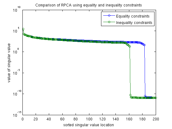
Compare the equality constrained version and the inequality constrained version. To do this, we can check whether the “L” components are really low rank and whether the “S” components are really sparse. Even if the two versions appear visually similar, the variables may behave quite differently with respect to low-rankness and sparsity.
fprintf('"S" from equality constrained version has \t%.1f%% nonzero entries\n',...
    100*nnz(SS_0)/numel(SS_0) );
fprintf('"S" from inequality constrained version has \t%.1f%% nonzero entries\n',...
    100*nnz(SS)/numel(SS) );

s  = svd(LL);    % inequality constraints
s0 = svd(LL_0);  % equality constraints

fprintf('"L" from equality constrained version has numerical rank\t %d (of %d possible)\n',...
    sum( s0>1e-6), min( m*n, nFrames)  );
fprintf('"L" from inequality constrained version has numerical rank\t %d (of %d possible)\n',...
    sum( s > 1e-6), min( m*n, nFrames)  );

figure();
semilogy( s0 ,'o-')
hold all;
semilogy( s ,'o-')
legend('Equality constraints','Inequality constraints');
xlabel('sorted singular value location');
ylabel('value of singular value');
title('Comparison of RPCA using equality and inequality constraints');
"S" from equality constrained version has  	21.7% nonzero entries
"S" from inequality constrained version has  	22.9% nonzero entries
"L" from equality constrained version has numerical rank	 183 (of 200 possible)
"L" from inequality constrained version has numerical rank	 161 (of 200 possible)
Published with MATLAB® 7.11